Quick start
Installation
You can easily install sympathor by running
python setup.py install
If needed, all dependencies can be found in requirements.txt.
A first example
We will show some features of sympathor by assuming the following use case: We have the race track of Spa-Franchorchamps given as an SVG drawing and are supposed to extract the circuit for a subsequent optimal control task of a race car. Note that this example can also be found in the folder example/racetrack.
Lucky us, we easily find a nice drawing of the circuit of Spa-Francorchamps on the internet:
 By Will Pittenger - Own work, CC BY-SA 3.0, link
Parsing
Without bothering about all the details like turns’ names or the pit lane, let’s fire up the parser of sympathor:
>>> from sympathor import ParsePaths
>>> paths = ParsePaths('examples/racetrack/Spa-Francorchamps.svg')
We can check the number of paths parsed and each path’s length with simple commands, like:
>>> len(paths)
39
>>> paths[0].length()
5164.234666618864
Going through all paths - most of them are of decorative nature, like circles, arrows, etc. - we find that the actual circuit is number 2 (the pit lane would be number 3, just saying):
>>> circuit = paths[2]
Sampling
Let’s sample the circuit …
>>> import numpy as np
>>> circuit_points = circuit.point(np.linspace(0, 1, 100))
… such that we can plot it:
>>> import matplotlib.pyplot as plt
>>> plt.plot(circuit_points[0, :], circuit_points[1, :], 'b.')
>>> plt.show()
Alrighty! There’s just one issue: the y-axis in SVGs is defined differently than how we normally plot things. It’s a good idea to flip the y-axis by default when depicting SVG paths:
>>> plt.plot(circuit_points[0, :], circuit_points[1, :], 'b.')
>>> plt.gca().invert_yaxis()
>>> plt.show()
Differential geometry
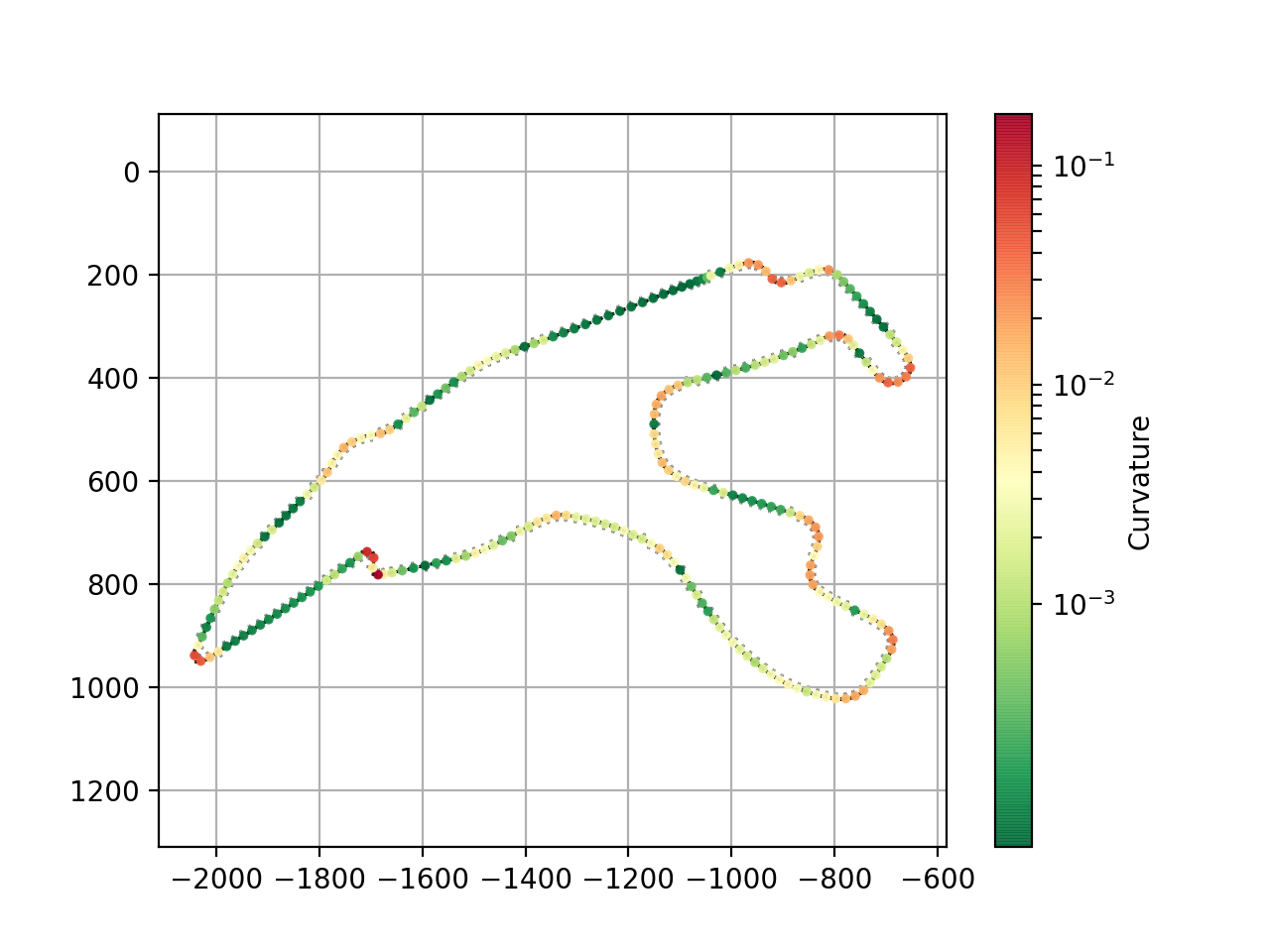
For our subsequent control task, we are asked to provide the Frenet frame at a certain (say, 250) number of samples, together with the curvature value. So let’s get those quantities:
>>> s = np.linspace(0, 1, 250)
>>> p = circuit.point(s)
>>> t = circuit.tangent(s)
>>> n = circuit.normal(s)
>>> c = circuit.curvature(s)
We’ll skip the code of plotting them since it’s a bit lengthy, but have a look at the example in examples/racetrack for details. The result looks like this:

And that’s all for now. We suggest you head over to the examples to get more insight - if you’ve got questions or issues, feel free to reach out in one way or another.